Benchmarks#

Performance Benchmarks#

Methodology#

Test Environment#

Python: 3.11
GPU: NVIDIA GeForce RTX 5090
CPU: Intel Core Ultra 9 285K
OS: Linux 6.11.0-29-generic

What We Measure#

Kernel Performance Only: All benchmarks measure only the core delay-and-sum beamforming kernel execution time. We explicitly exclude:

CPU↔GPU memory transfers (depends on PCIe bandwidth, motherboard, etc., and pre-/post-processing steps may keep data on the GPU)
JIT compilation (amortized over multiple function-calls)
Data format reshaping (varies by scanner or file format)
Pre-processing and post-processing steps (bit-unpacking, demodulation, clutter filtering, etc.; varies by ultrasound sequence)

The benchmark focuses on the most compute-/memory-bandwidth-intensive part of beamforming rather than system-specific overheads.

Benchmark Dataset#

We use PyMUST’s rotating-disk Doppler dataset as our primary benchmark:

128 receive elements (L7-4 linear array)
63,001 voxels (25mm × 25mm grid, 0.1mm spacing)
32 frames (temporal ensemble)

This represents a realistic ultrafast imaging workload, although it is a small microbenchmark compared to the 3D, high-channel count datasets we’re actually interested in.

The benchmark scripts use the following settings:

linear interpolation
f-number: 1.0

Performance Results#

Benchmark Results

Implementation	Median Runtime	Points/Second	“Mach factor”
mach (GPU)	0.23 ms	1.13 × 10¹²	6.5×
Speed-of-Sound (35mm)	1.5 ms		1×
vbeam (JAX/GPU)	3.6 ms	7.2 × 10¹⁰	0.42×
PyMUST (CPU)	67 ms	3.8 × 10⁹	0.022×

What does “beamforming at the speed of sound” even mean?#

The speed-of-sound (“Mach 1”), represents the theoretical minimum time required for ultrasound waves to travel to the deepest imaging point and back, multiplied by the number of frames in the dataset. This is specific to each imaging scenario. For our benchmark with PyMUST’s rotating-disk Doppler dataset:

Maximum imaging depth: 35 mm
Speed of sound in rotating disk: 1,480 m/s
Round-trip time: 2 × 0.035 m ÷ 1,480 m/s = 47 μs per frame
Total for 32 frames: 47.3 μs × 32 = 1.5 ms

mach’s processing time depends on various factors (see Computational Complexity), so the “Mach factor” description is specific to this benchmark.

Benchmark Reproduction#

All benchmarks can be reproduced using the included test suite:

# Run full benchmark suite
make benchmark

# Generate performance plots
uv run --group compare tests/plot_benchmark.py --output assets/benchmark-doppler_disk.svg
uv run --group compare tests/plot_benchmark.py --points-per-second --output assets/benchmark-doppler_disk_pps.svg

The benchmark job in our CI pipeline (test_gpu.yml) automatically runs these benchmarks across different commits, providing continuous performance monitoring.

CUDA Optimizations#

mach optimizes GPU memory access patterns to improve performance. For those interested in learning more about CUDA optimization, excellent resources include:

CUDA Crash Course by CoffeeBeforeArch
How CUDA Programming Works - CUDA Architect presentation on CUDA best-practices
Optimizing Parallel Reduction in CUDA - NVIDIA example of optimizing a different algorithm

Key Optimizations in mach#

1. Coalesced Memory Access#

Channel data organized as [n_receive_elements, n_samples, n_frames]
Frames dimension is contiguous for coalesced access to reduce global memory reads

2. Pre-computed Transmit Wavefront Arrivals#

Pre-compute transmit arrival times to amortize delay calculation across repeated kernel calls
However, cannot pre-compute the full transmit+receive delay matrix (like PyMUST) for large datasets: (would require transmits × voxels × channels x size(float) memory)

3. Shared Memory for Delay Tables#

Transmit-to-receive delays computed only once per voxel (not 32× for 32 frames)
Delay and apodization tables cached in shared memory
Reused across all frames for each voxel

Memory Bandwidth and Compute Utilization#

The current thread-block and L1-cache parameters were selected for an RTX4090 (Blackwell). These should work well across Blackwell Architecture GPUs.

If you’re wondering if different thread-block or L1-cache parameters might be better for your specific GPU, Nsight Compute can be helpful to identify bottlenecks.

Nsight Compute Profile Summary

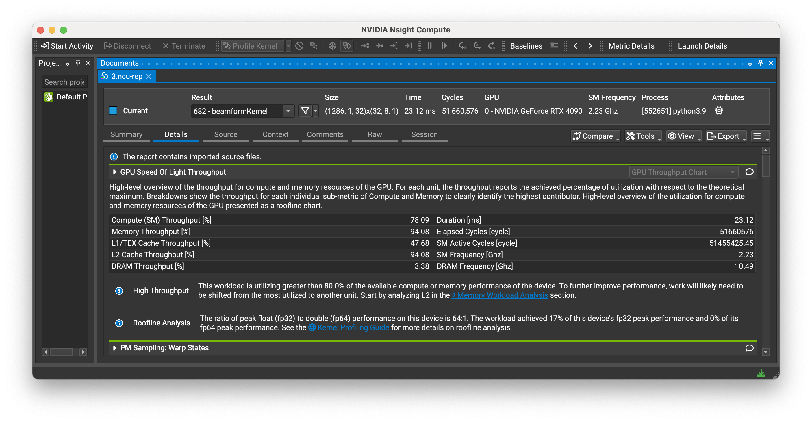
Figure: Nsight Compute profiling results shows 94% memory throughput and 78% compute throughput for the mach kernel on an RTX4090. (Different dataset)

Note: These utilization percentages are kernel-specific metrics from Nsight Compute, not the overall GPU utilization shown by nvidia-smi or nvtop.

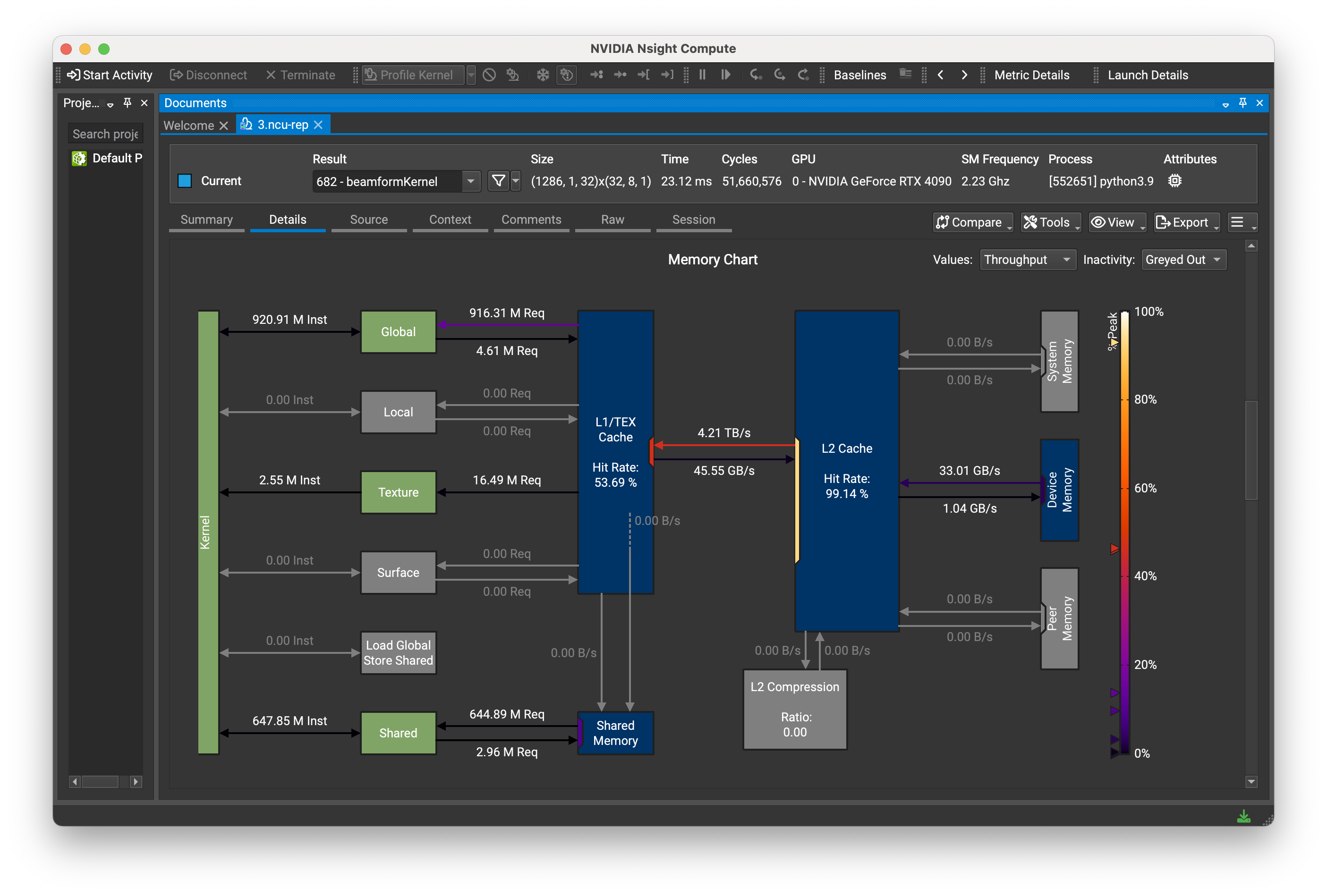
Nsight Compute memory workload analysis

Figure: Example Nsight Compute memory workload analysis. (Different dataset)

Anecdotally, kernel-duration seems to hit a pareto-optimum at >70% memory+compute-efficiency. Changing parameters at that point tends to trade-off memory/compute in a way that doesn’t change the overall kernel-time.

Scaling Performance#

Computational Complexity#

The beamforming algorithm scales as:

O(n_voxels × n_elements × n_frames)

For the PyMUST dataset: 63,001 voxels × 128 elements × 32 frames ≈ 2.6 × 10⁸ points

GPU Memory (VRAM) Usage#

mach allocates GPU memory only for input arguments and the output result; no intermediate arrays are created during computation, simplifying memory management.

Total GPU memory usage scales as:

O(n_voxels × n_frames + n_elements × n_samples × n_frames)

Where:

First term (n_voxels × n_frames): Output array size—dominates for large imaging grids
Second term (n_elements × n_samples × n_frames): Input data size—dominates for high-channel-count systems

Memory Usage Example#

Here is an example functional ultrasound imaging (fUSI) workload:

Imaging grid: 100×100×100 voxels (1M points)
Temporal frames: 200 frames
Matrix probe: 1024 elements
Samples per channel: 100
Data type: complex64 (8 bytes per sample)

Memory breakdown:

channel_data:       (1024, 100, 200) → 164 MB
rx_coords_m:        (1024, 3)        → 12 KB
scan_coords_m:      (1M, 3)          → 12 MB
tx_wave_arrivals_s: (1M,)            → 4 MB
out:                (1M, 200)        → 1.6 GB
                                    ─────────
Total GPU memory:                    ~1.78 GB

In this example, the output array (out) represents 90% of memory usage, demonstrating how large imaging grids dominate memory requirements for volumetric datasets.

Performance Scaling with Dataset Size#

Typical functional ultrasound imaging (fUSI) datasets we’re targeting:

1024+ receive elements (high-density arrays)
1M+ voxels (volumetric or high-resolution imaging)
100+ frames (longer temporal windows)

The performance scaling tests measure how mach’s beamforming performance scales with different dataset dimensions:

Voxel scaling: Testing grid resolution from 1e-4 (default) to 1e-5 meters (63k to 6.3M voxels)
Element scaling: Testing 1x to 64x receive elements (128 to 8,192 elements)
Frame scaling: Testing 1/32x to 16x ensemble size (1 to 512 frames)

To run the scaling benchmarks and then generate plots:

# Run pytest-benchmark
make benchmark

# Generate plots
python tests/plot_scaling.py --output assets/benchmark-scaling.svg

Benchmark scaling workload size

Figure: throughput is largely consistent across dataset sizes, except for a small decrease for <16 frames.

Performance Suggestions#

For Maximum Throughput:

Keep data on GPU: Use CuPy/JAX arrays to avoid CPU↔GPU transfers
Use sufficient ensemble size: Use ≥16 frames for complex64 or ≥32 frames for float32 to fully coalesce reads to global memory
Ensure contiguous frame dimension: The kernel requires frame-contiguous memory layouts.

Benchmarks

Contents