Note
Go to the end to download the full example code.
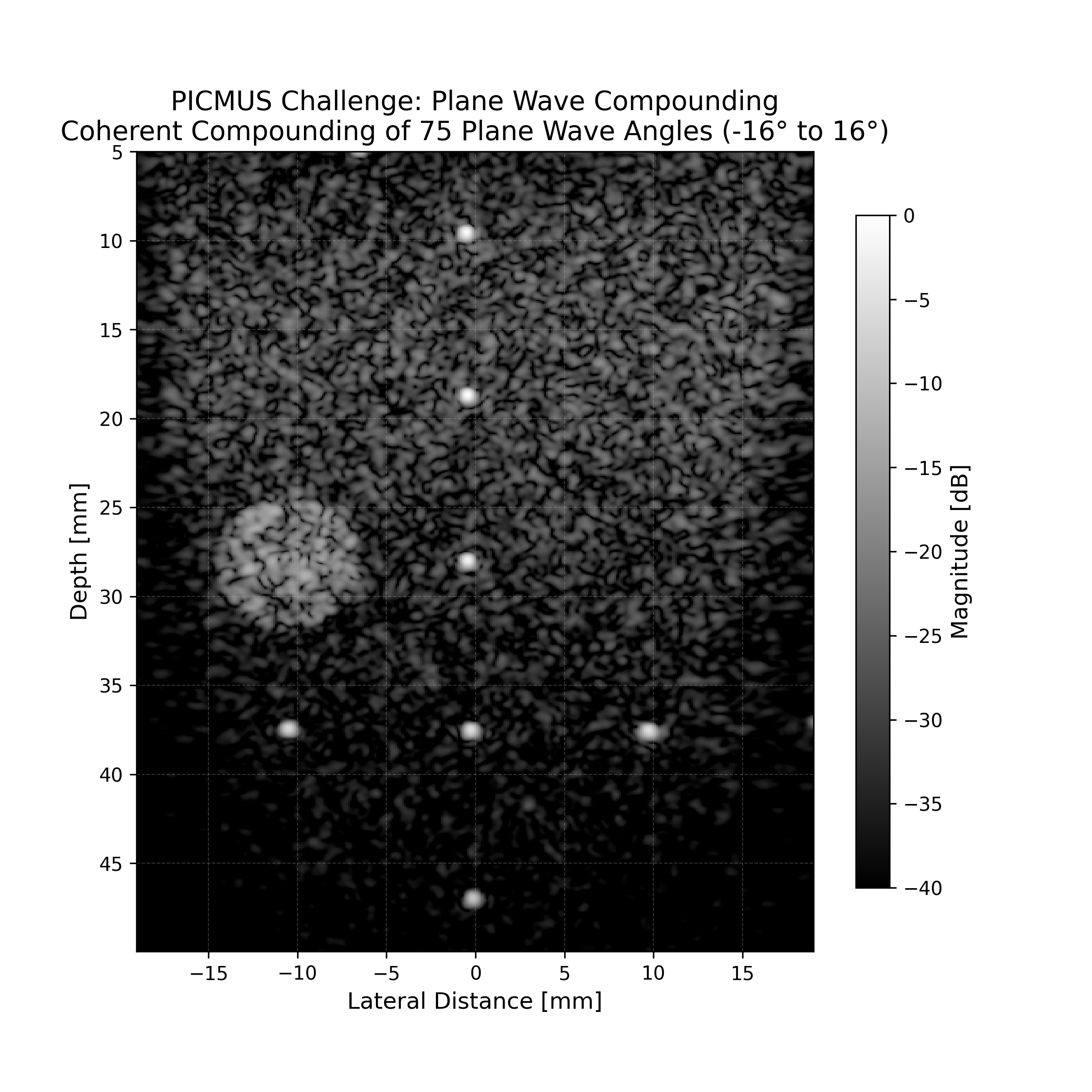
Plane Wave Compounding#
This example demonstrates plane wave compounding of data from the PICMUS challenge (Plane-wave Imaging Challenge in Medical Ultrasound). PICMUS provides standardized datasets for evaluating plane wave imaging algorithms.
Example overview:
Load ultrasound data from UFF format files
Beamform data from multiple plane-wave transmits
Coherently compound the results
Visualize the results
Attribution:
Example inspired by vbeam examples (magnusdk/vbeam)
Dataset from PICMUS challenge (https://www.creatis.insa-lyon.fr/Challenge/IEEE_IUS_2016/)
Note
To run this example, we recommend installing mach with all optional dependencies:
pip install mach-beamform[all]
This ensures all dependencies for the examples are available.
Import Required Libraries#
Let’s start by importing the necessary libraries.
import hashlib

import matplotlib.pyplot as plt
import numpy as np

# Import mach modules
from mach import experimental
from mach._vis import db_zero
from mach.io.uff import create_beamforming_setup
from mach.io.utils import cached_download

try:
    from pyuff_ustb import Uff
except ImportError as err:
    raise ImportError("⚠️  pyuff_ustb is required for UFF data loading. Install with: pip install pyuff-ustb") from err

# Convenience constants
MM_PER_METER = 1000
Download PICMUS Challenge Dataset#
The PICMUS challenge contains multiple datasets with multi-angle plane-wave transmits. This example uses the resolution dataset, which features:
128-element linear array at 5.2 MHz center frequency
75 plane wave transmits at angles from -16° to +16°
Point targets and cysts for resolution and contrast assessment
print("📂 Downloading PICMUS challenge dataset...")

# Download the UFF data file (cached locally after first download)
# Source: https://unioslo.github.io/USTB/datasets.html
url = "https://zenodo.org/records/20261898/files/PICMUS_experiment_resolution_distortion.uff"
uff_path = cached_download(
    url,
    expected_size=145_518_524,
    expected_hash="c93af0781daeebf771e53a42a629d4f311407410166ef2f1d227e9d2a1b8c641",
    digest=hashlib.sha256,
    filename="PICMUS_experiment_resolution_distortion.uff",
)

print(f"✓ Dataset downloaded to: {uff_path}")
print(f"  File size: {uff_path.stat().st_size / 1e6:.1f} MB")
📂 Downloading PICMUS challenge dataset...

Downloading PICMUS_experiment_resolution_distortion.uff:   0%|          | 0.00/146M [00:00<?, ?B/s]
Downloading PICMUS_experiment_resolution_distortion.uff:   1%|          | 1.05M/146M [00:01<02:56, 817kB/s]
Downloading PICMUS_experiment_resolution_distortion.uff:   1%|▏         | 2.10M/146M [00:01<01:38, 1.46MB/s]
Downloading PICMUS_experiment_resolution_distortion.uff:   2%|▏         | 3.15M/146M [00:01<01:02, 2.26MB/s]
Downloading PICMUS_experiment_resolution_distortion.uff:   3%|▎         | 4.19M/146M [00:01<00:46, 3.05MB/s]
Downloading PICMUS_experiment_resolution_distortion.uff:   4%|▎         | 5.24M/146M [00:02<00:37, 3.79MB/s]
Downloading PICMUS_experiment_resolution_distortion.uff:   5%|▌         | 7.34M/146M [00:02<00:23, 5.92MB/s]
Downloading PICMUS_experiment_resolution_distortion.uff:   7%|▋         | 10.5M/146M [00:02<00:14, 9.29MB/s]
Downloading PICMUS_experiment_resolution_distortion.uff:   9%|▉         | 13.6M/146M [00:02<00:10, 12.0MB/s]
Downloading PICMUS_experiment_resolution_distortion.uff:  12%|█▏        | 17.8M/146M [00:02<00:08, 15.7MB/s]
Downloading PICMUS_experiment_resolution_distortion.uff:  15%|█▌        | 22.0M/146M [00:02<00:06, 18.4MB/s]
Downloading PICMUS_experiment_resolution_distortion.uff:  18%|█▊        | 26.2M/146M [00:03<00:05, 20.5MB/s]
Downloading PICMUS_experiment_resolution_distortion.uff:  20%|██        | 29.4M/146M [00:03<00:05, 20.2MB/s]
Downloading PICMUS_experiment_resolution_distortion.uff:  22%|██▏       | 32.5M/146M [00:03<00:05, 20.0MB/s]
Downloading PICMUS_experiment_resolution_distortion.uff:  25%|██▌       | 36.7M/146M [00:03<00:05, 21.6MB/s]
Downloading PICMUS_experiment_resolution_distortion.uff:  28%|██▊       | 40.9M/146M [00:03<00:04, 22.8MB/s]
Downloading PICMUS_experiment_resolution_distortion.uff:  30%|███       | 44.0M/146M [00:03<00:04, 21.7MB/s]
Downloading PICMUS_experiment_resolution_distortion.uff:  33%|███▎      | 48.2M/146M [00:04<00:04, 22.8MB/s]
Downloading PICMUS_experiment_resolution_distortion.uff:  35%|███▌      | 51.4M/146M [00:04<00:04, 21.8MB/s]
Downloading PICMUS_experiment_resolution_distortion.uff:  38%|███▊      | 55.6M/146M [00:04<00:03, 23.0MB/s]
Downloading PICMUS_experiment_resolution_distortion.uff:  40%|████      | 58.7M/146M [00:04<00:03, 21.9MB/s]
Downloading PICMUS_experiment_resolution_distortion.uff:  43%|████▎     | 62.9M/146M [00:04<00:03, 23.0MB/s]
Downloading PICMUS_experiment_resolution_distortion.uff:  45%|████▌     | 66.1M/146M [00:04<00:03, 21.9MB/s]
Downloading PICMUS_experiment_resolution_distortion.uff:  48%|████▊     | 69.2M/146M [00:05<00:03, 21.2MB/s]
Downloading PICMUS_experiment_resolution_distortion.uff:  50%|█████     | 73.4M/146M [00:05<00:03, 22.5MB/s]
Downloading PICMUS_experiment_resolution_distortion.uff:  53%|█████▎    | 77.6M/146M [00:05<00:02, 23.4MB/s]
Downloading PICMUS_experiment_resolution_distortion.uff:  56%|█████▌    | 81.8M/146M [00:05<00:02, 24.1MB/s]
Downloading PICMUS_experiment_resolution_distortion.uff:  58%|█████▊    | 84.9M/146M [00:05<00:02, 22.8MB/s]
Downloading PICMUS_experiment_resolution_distortion.uff:  61%|██████    | 89.1M/146M [00:05<00:02, 23.6MB/s]
Downloading PICMUS_experiment_resolution_distortion.uff:  64%|██████▍   | 93.3M/146M [00:05<00:02, 24.2MB/s]
Downloading PICMUS_experiment_resolution_distortion.uff:  66%|██████▋   | 96.5M/146M [00:06<00:02, 22.8MB/s]
Downloading PICMUS_experiment_resolution_distortion.uff:  69%|██████▉   | 101M/146M [00:06<00:01, 23.6MB/s]
Downloading PICMUS_experiment_resolution_distortion.uff:  72%|███████▏  | 105M/146M [00:06<00:01, 24.2MB/s]
Downloading PICMUS_experiment_resolution_distortion.uff:  75%|███████▍  | 109M/146M [00:06<00:01, 24.7MB/s]
Downloading PICMUS_experiment_resolution_distortion.uff:  77%|███████▋  | 112M/146M [00:06<00:01, 23.1MB/s]
Downloading PICMUS_experiment_resolution_distortion.uff:  79%|███████▉  | 115M/146M [00:06<00:01, 22.0MB/s]
Downloading PICMUS_experiment_resolution_distortion.uff:  82%|████████▏ | 120M/146M [00:07<00:01, 23.0MB/s]
Downloading PICMUS_experiment_resolution_distortion.uff:  85%|████████▌ | 124M/146M [00:07<00:00, 23.6MB/s]
Downloading PICMUS_experiment_resolution_distortion.uff:  88%|████████▊ | 128M/146M [00:07<00:00, 24.1MB/s]
Downloading PICMUS_experiment_resolution_distortion.uff:  91%|█████████ | 132M/146M [00:07<00:00, 24.4MB/s]
Downloading PICMUS_experiment_resolution_distortion.uff:  93%|█████████▎| 135M/146M [00:07<00:00, 22.9MB/s]
Downloading PICMUS_experiment_resolution_distortion.uff:  95%|█████████▌| 138M/146M [00:07<00:00, 21.9MB/s]
Downloading PICMUS_experiment_resolution_distortion.uff:  98%|█████████▊| 143M/146M [00:08<00:00, 23.1MB/s]
Downloading PICMUS_experiment_resolution_distortion.uff: 100%|██████████| 146M/146M [00:08<00:00, 21.5MB/s]
Downloading PICMUS_experiment_resolution_distortion.uff: 100%|██████████| 146M/146M [00:08<00:00, 17.6MB/s]
✓ Dataset downloaded to: /home/runner/.cache/mach/PICMUS_experiment_resolution_distortion.uff
  File size: 145.5 MB
Load and Inspect PICMUS Data#
UFF files contain structured ultrasound data including channel data (RF signals), probe geometry, and scan parameters. Let’s examine the PICMUS dataset structure.
print("\n📋 Loading PICMUS data structure...")

# Open UFF file and extract components
uff_file = Uff(str(uff_path))
channel_data = uff_file.read("/channel_data")
scan = uff_file.read("/scan")

# Display challenge dataset information
print("\n📊 PICMUS Challenge Dataset:")
print(f"   Plane wave transmits: {len(channel_data.sequence)}")
print(f"   Array elements: {channel_data.probe.N}")
print(f"   Samples per acquisition: {channel_data.data.shape[0]}")
print(f"   Frames: {channel_data.data.shape[-1] if channel_data.data.ndim > 3 else 1}")
print(f"   Sampling frequency: {channel_data.sampling_frequency / 1e6:.1f} MHz")
print(f"   Center frequency: {channel_data.modulation_frequency / 1e6:.1f} MHz")
print(f"   Speed of sound: {channel_data.sound_speed} m/s")

# Display plane wave transmit angles
angles_deg = [np.rad2deg(wave.source.azimuth) for wave in channel_data.sequence]
print(f"   Plane wave angles: {min(angles_deg):.1f}° to {max(angles_deg):.1f}°")
print(f"   Angular step: {np.diff(angles_deg)[0]:.1f}°")

# Display imaging region
print("\n🎯 Imaging Region:")
print(f"   Lateral samples: {scan.x_axis.size}")
print(f"   Depth samples: {scan.z_axis.size}")
print(f"   Lateral extent: {scan.x_axis.min() * MM_PER_METER:.1f} to {scan.x_axis.max() * MM_PER_METER:.1f} mm")
print(f"   Depth extent: {scan.z_axis.min() * MM_PER_METER:.1f} to {scan.z_axis.max() * MM_PER_METER:.1f} mm")
📋 Loading PICMUS data structure...

📊 PICMUS Challenge Dataset:
   Plane wave transmits: 75
   Array elements: 128
   Samples per acquisition: 3328
   Frames: 1
   Sampling frequency: 20.8 MHz
   Center frequency: 0.0 MHz
   Speed of sound: 1540.0 m/s
   Plane wave angles: -16.0° to 16.0°
   Angular step: 0.4°

🎯 Imaging Region:
   Lateral samples: 387
   Depth samples: 609
   Lateral extent: -19.1 to 19.0 mm
   Depth extent: 5.0 to 49.9 mm
Extract metadata for mach#
print("\n🔄 Preparing data for beamforming...")

# Create beamforming setup for all plane wave angles
beamform_kwargs = create_beamforming_setup(
    channel_data=channel_data,
    scan=scan,
    f_number=1.7,
)

print("📊 Beamforming setup:")
print(f"   Sensor data shape: {beamform_kwargs['channel_data'].shape}")
print("   (transmits, elements, samples, frames)")
print(f"   Output points: {beamform_kwargs['scan_coords_m'].shape[0]:,}")
print(f"   Transmit arrivals shape: {beamform_kwargs['tx_wave_arrivals_s'].shape}")
print(f"   F-number: {beamform_kwargs['f_number']}")

# Extract number of plane-wave transmits
n_transmits = beamform_kwargs["channel_data"].shape[0]
print(f"   Beamforming {n_transmits} plane-wave transmits")
🔄 Preparing data for beamforming...
📊 Beamforming setup:
   Sensor data shape: (75, 128, 3328, 1)
   (transmits, elements, samples, frames)
   Output points: 235,683
   Transmit arrivals shape: (75, 235683)
   F-number: 1.7
   Beamforming 75 plane-wave transmits
Beamform and compound#
Now we beamform and compound the data:
Individual beamforming: Apply delay-and-sum beamforming to each plane-wave transmit
Coherent compounding: Sum the results to form the final image
Note: The mach.experimental API is subject to change.
print("\n🚀 Beamforming and compounding...")

result = experimental.beamform(**beamform_kwargs)

print("✓ Beamforming and compounding completed!")
print(f"  Output shape: {result.shape} (points, frames)")
print(f"  Data type: {result.dtype}")
print(f"  Coherently compounded {n_transmits} plane-wave transmits")
🚀 Beamforming and compounding...
/home/runner/work/mach/mach/src/mach/kernel.py:254: UserWarning: array is not contiguous, rearranging will add latency
  channel_data = ensure_contiguous(channel_data)
/home/runner/work/mach/mach/src/mach/kernel.py:277: UserWarning: Found 4 input array(s) on CPU. This will add latency due to CPU<->GPU memory transfers. For optimal performance with CUDA beamforming, move arrays to GPU using cupy, jax, or similar.
  nb_beamform(  # ty: ignore[no-matching-overload]
✓ Beamforming and compounding completed!
  Output shape: (235683, 1) (points, frames)
  Data type: complex64
  Coherently compounded 75 plane-wave transmits
Reshape results#
The beamformed data needs to be reshaped to the 2D imaging grid.
print("\n📊 Processing compounded results...")

# Reshape from flattened points back to 2D imaging grid
grid_shape = (scan.x_axis.size, scan.z_axis.size)
beamformed_image = result.reshape(grid_shape)

# Extract magnitude for B-mode display (envelope detection)
bmode_image = np.abs(beamformed_image)

print("✓ Image processing complete")
print(f"  Image shape: {bmode_image.shape} (lateral, depth)")
print(f"  Dynamic range: {bmode_image.min():.2e} to {bmode_image.max():.2e}")
📊 Processing compounded results...
✓ Image processing complete
  Image shape: (387, 609) (lateral, depth)
  Dynamic range: 2.82e-03 to 8.00e+01
Visualize B-Mode#
print("\n📊 Visualizing B-mode...")

# Convert to logarithmic (dB) scale for display
bmode_db = db_zero(beamformed_image)

# Create high-quality visualization
fig, ax = plt.subplots(figsize=(8, 8), dpi=300)

# Set up coordinate system for proper display
extent = [
    scan.x_axis.min() * MM_PER_METER,
    scan.x_axis.max() * MM_PER_METER,
    scan.z_axis.max() * MM_PER_METER,
    scan.z_axis.min() * MM_PER_METER,
]

# Display the compounded image
im = ax.imshow(
    bmode_db.T,
    cmap="gray",  # Clinical grayscale colormap
    vmin=-40,  # 40 dB dynamic range
    vmax=0,  # Normalized to maximum
    extent=extent,  # Physical coordinates in mm
    aspect="equal",  # Preserve spatial relationships
    origin="upper",  # Depth increases downward (standard)
    interpolation="nearest",  # Preserve sharp phantom features
)

# Add comprehensive labeling
ax.set_title(
    f"PICMUS Challenge: Plane Wave Compounding\n"
    f"Coherent Compounding of {n_transmits} Plane Wave Angles "
    f"({min(angles_deg):.0f}° to {max(angles_deg):.0f}°)",
    fontsize=14,
)
ax.set_xlabel("Lateral Distance [mm]", fontsize=12)
ax.set_ylabel("Depth [mm]", fontsize=12)

# Add colorbar with proper formatting
cbar = plt.colorbar(im, ax=ax, shrink=0.8)
cbar.set_label("Magnitude [dB]", fontsize=12)
cbar.ax.tick_params(labelsize=10)

# Add subtle grid for better readability
ax.grid(True, alpha=0.3, linestyle="--", linewidth=0.5)
📊 Visualizing B-mode...
Expected results#
The plane wave compounded image should clearly resolve:
Point targets: Sharp, well-defined spots for lateral/axial resolution measurement
Hyperechoic lesion: Bright circle to test for geometric distortion
Uniform speckle: Consistent background texture in tissue-mimicking regions
Total running time of the script: (0 minutes 11.292 seconds)