Note

Go to the end to download the full example code.

Doppler#

This example demonstrates CUDA-accelerated ultrasound beamforming for power Doppler imaging using a rotating disk phantom dataset. We’ll use the same dataset as the PyMUST Doppler example and follow a similar workflow to the ultraspy doppler tutorial.

Dataset Attribution: The rotating disk data comes from PyMUST’s example dataset [1], which contains ultrasound data from a tissue-mimicking phantom with a rotating disk that creates Doppler shifts. This is the same dataset used in the MUST/PyMUST tutorials.

Key Learning Objectives:

Load and inspect ultrasound RF data from PyMUST
Convert RF signals to IQ (in-phase/quadrature) format
Set up imaging geometry for plane wave beamforming
Perform CUDA-accelerated delay-and-sum beamforming
Compute power Doppler images for motion detection
Visualize beamformed results

The power Doppler technique is particularly useful for detecting slow flow and motion by analyzing the variance in the ultrasound signal over time.

References#

Import Required Libraries#

Let’s start by importing all the necessary libraries and checking dependencies.

import matplotlib.pyplot as plt
import numpy as np
from einops import rearrange

# Import mach modules
from mach import wavefront
from mach._vis import db_zero
from mach.io.must import (
    download_pymust_doppler_data,
    extract_pymust_params,
    linear_probe_positions,
    scan_grid,
)
from mach.kernel import beamform

# Check for PyMUST dependency
try:
    import pymust
except ImportError as err:
    raise ImportError("⚠️  PyMUST is currently required for RF-to-IQ demodulation.") from err

# Convenience constant
MM_PER_METER = 1000

Load PyMUST Rotating Disk Dataset#

First, we’ll download and inspect the PyMUST rotating disk dataset. This dataset contains RF data from a tissue-mimicking phantom with a rotating disk, which creates controlled Doppler shifts useful for validating beamforming algorithms.

The dataset parameters match those used in the original PyMUST examples: - 128-element linear array at 5 MHz center frequency - 32 plane wave acquisitions at 10 kHz PRF - Rotating disk phantom creating known Doppler patterns

print("📂 Loading PyMUST rotating disk data...")

# Download the dataset (cached locally after first download)
mat_data = download_pymust_doppler_data()
params = extract_pymust_params(mat_data)

# Display dataset information
print("\n📋 Dataset Information:")
print(f"   Samples (fast time): {mat_data['RF'].shape[0]}")
print(f"   Elements: {params['Nelements']}")
print(f"   Frames (slow time): {mat_data['RF'].shape[2]}")
print(f"   Sample rate: {params['fs'] / 1e6:.1f} MHz")
print(f"   Center frequency: {params['fc'] / 1e6:.1f} MHz")
print(f"   Speed of sound: {params['c']} m/s")
print(f"   PRF: {params['PRF']} Hz")

📂 Loading PyMUST rotating disk data...

📋 Dataset Information:
   Samples (fast time): 334
   Elements: 128
   Frames (slow time): 32
   Sample rate: 6.7 MHz
   Center frequency: 5.0 MHz
   Speed of sound: 1480 m/s
   PRF: 10000 Hz

Convert RF Data to IQ Format#

For Doppler processing, we need to work with complex-valued IQ (in-phase/quadrature) data rather than real-valued RF signals. This conversion preserves phase information essential for Doppler velocity estimation.

Following the PyMUST workflow, we use their rf2iq function for consistency with reference implementations.

print("\n🔄 Converting RF data to IQ format...")

# Convert RF to IQ using PyMUST's method
# This performs baseband demodulation around the center frequency
rf_data = mat_data["RF"].astype(float)
iq_data = pymust.rf2iq(rf_data, params)

print("✓ IQ conversion complete")
print(f"  IQ data shape: {iq_data.shape} (samples, elements, frames)")
print(f"  Data type: {iq_data.dtype}")

🔄 Converting RF data to IQ format...
✓ IQ conversion complete
  IQ data shape: (334, 128, 32) (samples, elements, frames)
  Data type: complex128

Set Up Imaging Geometry#

Next, we’ll define the imaging geometry including: - Linear array element positions - 2D imaging grid spanning the region of interest - Transmit delay pattern for 0° plane wave imaging

We use the same grid parameters as the original PyMUST example for consistency.

print("\n📐 Setting up imaging geometry...")

# Create linear array element positions
element_positions = linear_probe_positions(params["Nelements"], params["pitch"])
print("📍 Linear Array Configuration:")
print(f"   Elements: {len(element_positions)}")
print(f"   Pitch: {params['pitch'] * MM_PER_METER:.2f} mm")
print(f"   Total aperture: {np.ptp(element_positions[:, 0]) * MM_PER_METER:.1f} mm")

# Create 2D imaging grid matching PyMUST example
# Grid spans ±12.5 mm laterally and 10-35 mm in depth
x = np.linspace(-12.5e-3, 12.5e-3, num=251, endpoint=True)
y = np.array([0.0])  # 2D imaging (single y-plane)
z = np.linspace(10e-3, 35e-3, num=251, endpoint=True)

# Convert to flattened grid points for beamforming
grid_points = scan_grid(x, y, z)

print("🎯 Imaging Grid:")
print(f"   Grid points: {grid_points.shape[0]:,}")
print(f"   Lateral extent: {x.min() * MM_PER_METER:.1f} to {x.max() * MM_PER_METER:.1f} mm")
print(f"   Depth extent: {z.min() * MM_PER_METER:.1f} to {z.max() * MM_PER_METER:.1f} mm")

📐 Setting up imaging geometry...
📍 Linear Array Configuration:
   Elements: 128
   Pitch: 0.30 mm
   Total aperture: 37.8 mm
🎯 Imaging Grid:
   Grid points: 63,001
   Lateral extent: -12.5 to 12.5 mm
   Depth extent: 10.0 to 35.0 mm

Compute Transmit Delay Pattern#

For plane wave imaging, we need to compute the transmit delays that define when the transmitted wavefront arrives at each imaging point. Here we use a 0° plane wave (normal incidence) as in the PyMUST example.

# Compute transmit delays for 0° plane wave
# The plane wave propagates in the +z direction (into the medium)
wavefront_arrivals_s = (
    wavefront.plane(
        origin_m=np.array([0, 0, 0]),  # Wave originates at array face
        points_m=grid_points,  # All grid points
        direction=np.array([0, 0, 1]),  # +z direction (0° angle)
    )
    / params["c"]  # Convert to time delays
)

print("⏱️  Transmit Delays:")
print("   Pattern: 0° plane wave")
print(
    f"   Wavefront arrival ranges from: {wavefront_arrivals_s.min() * 1e6:.1f} to {wavefront_arrivals_s.max() * 1e6:.1f} μs"
)

⏱️  Transmit Delays:
   Pattern: 0° plane wave
   Wavefront arrival ranges from: 6.8 to 23.6 μs

Prepare Data for GPU Beamforming#

mach expects data in a specific format: - IQ data: (elements, samples, frames) - All arrays as contiguous float32/complex64

We’ll reorder the PyMUST data to match this expected format.

# Reorder IQ data: (samples, elements, frames) -> (elements, samples, frames)
iq_data_reordered = np.ascontiguousarray(
    rearrange(iq_data, "samples elements frames -> elements samples frames"), dtype=np.complex64
)

print("📊 Data Preparation Complete:")
print(f"   IQ data shape: {iq_data_reordered.shape} (elements, samples, frames)")
print(f"   Element positions: {element_positions.shape} (elements, xyz)")
print(f"   Output grid points: {grid_points.shape[0]:,}")
print(f"   Data size: ~{iq_data_reordered.nbytes / 1e6:.1f} MB")

📊 Data Preparation Complete:
   IQ data shape: (128, 334, 32) (elements, samples, frames)
   Element positions: (128, 3) (elements, xyz)
   Output grid points: 63,001
   Data size: ~10.9 MB

Perform GPU Beamforming#

Now we’ll run the GPU-accelerated delay-and-sum beamforming. The mach kernel efficiently handles: - Dynamic receive focusing with configurable f-number - Time-gain compensation and apodization - Complex IQ processing for phase-sensitive applications

This single call processes all frames simultaneously on the GPU.

print("\n🚀 Running GPU beamforming...")

# Run CUDA beamforming with parameters from PyMUST dataset
result = beamform(
    channel_data=iq_data_reordered,  # IQ data from all elements
    rx_coords_m=element_positions,  # Array element positions
    scan_coords_m=grid_points,  # Imaging grid coordinates
    tx_wave_arrivals_s=wavefront_arrivals_s,  # Transmit arrival times (s)
    f_number=float(params["fnumber"]),  # Dynamic focusing f-number
    rx_start_s=float(params["t0"]),  # Data acquisition start time
    sampling_freq_hz=float(params["fs"]),  # Sampling frequency
    sound_speed_m_s=float(params["c"]),  # Medium sound speed
    modulation_freq_hz=float(params["fc"]),  # Demodulation frequency
    tukey_alpha=0.0,  # No additional windowing
)

print("✓ GPU beamforming completed!")
print(f"  Output shape: {result.shape} (grid_points, frames)")
print(f"  Data type: {result.dtype}")

🚀 Running GPU beamforming...
/home/runner/work/mach/mach/src/mach/kernel.py:236: UserWarning: Found 5 input array(s) on CPU. This will add latency due to CPU<->GPU memory transfers. For optimal performance with CUDA beamforming, move arrays to GPU using cupy, jax, or similar.
  nb_beamform(
✓ GPU beamforming completed!
  Output shape: (63001, 32) (grid_points, frames)
  Data type: complex64

Compute Power Doppler Image#

Power Doppler imaging detects motion by analyzing signal variance over time. Unlike color Doppler which estimates velocity, power Doppler is sensitive to any motion regardless of direction, making it excellent for detecting slow flow.

We compute the temporal power by summing the squared magnitude across frames.

print("\n📊 Computing power Doppler image...")

# Calculate power Doppler as sum of squared magnitudes over time
# This is a basic power Doppler - more sophisticated methods could include:
# - SVD-based clutter filtering
# - Temporal smoothing
# - Motion-adaptive processing
power_doppler = np.square(np.abs(result)).sum(axis=-1)

# Reshape back to 2D grid for visualization
power_doppler_2d = power_doppler.reshape(len(x), len(z))

print("✓ Power Doppler computation complete")
print(f"  Image shape: {power_doppler_2d.shape} (lateral, depth)")
print(f"  Dynamic range: {power_doppler_2d.min():.2e} to {power_doppler_2d.max():.2e}")

📊 Computing power Doppler image...
✓ Power Doppler computation complete
  Image shape: (251, 251) (lateral, depth)
  Dynamic range: 2.16e+04 to 7.29e+09

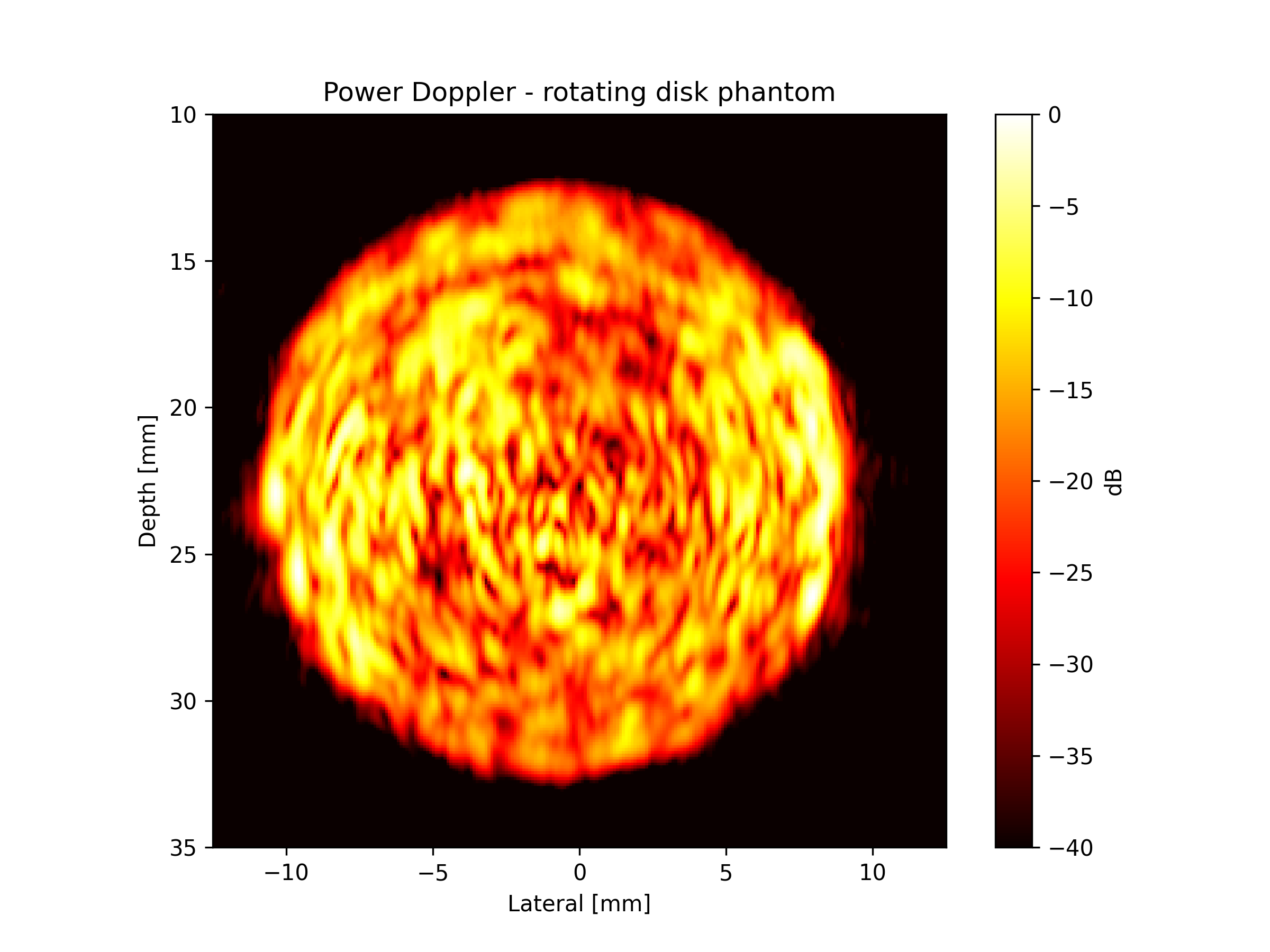
Visualize Power Doppler Results#

Finally, let’s create a publication-quality visualization of our power Doppler image. We’ll use a logarithmic scale (dB) for better contrast, similar to clinical ultrasound displays.

The rotating disk should appear as a bright circular region indicating motion, while static background remains dark.

print("\n📊 Creating visualization...")

# Convert to dB scale for better visualization
power_doppler_db = db_zero(power_doppler_2d)

# Plot along with axis labels
fig, ax = plt.subplots(figsize=(8, 6), dpi=300)
extent = [x.min() * MM_PER_METER, x.max() * MM_PER_METER, z.max() * MM_PER_METER, z.min() * MM_PER_METER]
im = ax.imshow(
    power_doppler_db.T,
    cmap="hot",
    vmax=0,  # Normalized to maximum
    vmin=-40,  # 40 dB dynamic range
    extent=extent,  # Physical coordinates
    aspect="equal",
    origin="upper",  # Standard ultrasound orientation
)
ax.set_title("Power Doppler - rotating disk phantom")
ax.set_xlabel("Lateral [mm]")
ax.set_ylabel("Depth [mm]")

# Add colorbar with proper labeling
cbar = fig.colorbar(im, ax=ax)
cbar.set_label("dB")

plt.show()

📊 Creating visualization...

Results Summary and Discussion#

Expected results: The power Doppler image should show: - Bright circular region: The rotating disk creates motion that appears bright - Dark background: Static tissue appears dark in power Doppler - Spatial accuracy: Disk location matches the physical phantom geometry - Matches: https://www.biomecardio.com/MUST/functions/html/iq2doppler_doc.html#7

Performance advantages: GPU beamforming with mach provides significant speedup over CPU implementations while maintaining numerical accuracy comparable to reference methods like PyMUST.

Next steps: This example provides a foundation for more advanced Doppler processing: - Advanced clutter filtering (SVD, polynomial regression) - 3D power Doppler

Total running time of the script: (0 minutes 1.056 seconds)

Gallery generated by Sphinx-Gallery

Doppler

Contents

Doppler#

References#

Import Required Libraries#

Load PyMUST Rotating Disk Dataset#

Convert RF Data to IQ Format#

Set Up Imaging Geometry#

Compute Transmit Delay Pattern#

Prepare Data for GPU Beamforming#

Perform GPU Beamforming#

Compute Power Doppler Image#

Visualize Power Doppler Results#

Results Summary and Discussion#